AC Linear optimal power flow time series¶

General indices and dimensions

Variable	Description
n	Number of nodes
m	Number of branches
ng	Number of generators
nb	Number of batteries
nl	Number of loads
nt	Number of time steps
pqpv	Vector of node indices of the the PQ and PV buses.
vd	Vector of node indices of the the Slack (or VD) buses.

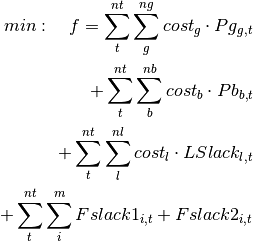
Objective function¶

The objective function minimizes the cost of generation plus all the slack variables set in the problem.

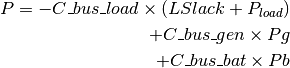
$min: \quad f = \sum_t^{nt} \sum_g^{ng} cost_g \cdot Pg_{g,t} \\ + \sum_t^{nt} \sum_b^{nb} cost_b \cdot Pb_{b, t} \\ + \sum_t^{nt} \sum_l^{nl} cost_l \cdot LSlack_{l, t} \\ + \sum_t^{nt} \sum_i^{m} Fslack1_{i,t} + Fslack2_{i,t} \\$

Power injections¶

This equation is not a restriction but the computation of the power injections (fix and LP variables) that are injected per node, such that the vector $P$ is dimensionally coherent with the number of buses.

$P = - C\_bus\_load \times (LSlack + P_{load}) \\ + C\_bus\_gen \times Pg \\ + C\_bus\_bat \times Pb$

$Q = - C\_bus\_load \times (LSlack + Q_{load})$

Variable	Description	Dimensions	Type	Units
$P$	Matrix of active power per node and time step.	n, nt	Float + LP	p.u.
$C\_bus\_gen$	Bus-Generators connectivity matrix.	n, ng	int	1/0
$Pg$	Matrix of generators active power per time step.	ng, nt	LP	p.u.
$C\_bus\_bat$	Bus-Batteries connectivity matrix.	nb	int	1/0
$Pb$	Matrix of batteries active power per time step.	nb, nt	LP	p.u.
$C\_bus\_load$	Bus-Generators connectivity matrix.	n, nl	int	1/0
$P_{load}$	Matrix of active power loads per time step.	nl, nt	Float	p.u.
$Q_{load}$	Matrix of reactive power loads per time step.	nl, nt	Float	p.u.
$LSlack$	Matrix of active power load slack variables per time step.	nl, nt	LP	p.u.

Nodal power balance¶

This is the OPF based on the formulation presented in Linearized AC Load Flow Applied to Analysis in Electric Power Systems [1], we obtain a way to solve circuits in one shot (without iterations) and with quite positive results for a linear approximation.

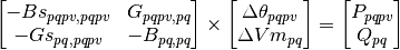
$\begin{bmatrix} -Bs_{pqpv, pqpv} & G_{pqpv, pq} \\ -Gs_{pq, pqpv} & -B_{pq,pq} \\ \end{bmatrix} \times \begin{bmatrix} \Delta \theta_{pqpv}\\ \Delta Vm_{pq}\\ \end{bmatrix} = \begin{bmatrix} P_{pqpv}\\ Q_{pq}\\ \end{bmatrix}$

This matrix equation turns into two sets of restrictions:

$-Bs_{pqpv, pqpv} \times \Delta \theta_{pqpv} + G_{pqpv, pq} \times \Delta Vm_{pq} = P_{pqpv}$

$-Gs_{pq, pqpv} \times \Delta \theta_{pqpv} - B_{pq,pq} \times \Delta Vm_{pq} = Q_{pq}$

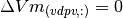
An additional set of restrictions is needed in order to include the slack nodes in the formulation. These are not required for the power flow formulation but they are in the optimal power flow one that is presented.

$-Bs_{vd, :} \times \Delta \theta + G_{vd, :} \times \Delta Vm = P_{vd}$

Remember to set the slack-node voltage angles and module increments and the PV node voltage module increments to zero! Otherwise the generator’s power will no be used by the solver to provide voltage values.

$\Delta\theta_{(vd, :)} = 0$

$\Delta Vm_{(vdpv, :)} = 0$

Variable	Description	Dimensions	Type	Units
$B$	Matrix of susceptances. $Im\{Y\}$ .	n, n	Float	p.u.
$Bs$	Matrix of susceptances of the series elements. $Im \left\{Y_{series} \right\}$ .	n, n	Float	p.u.
$G$	Matrix of conductances. $Re\{Y\}$ .	n, n	Float	p.u.
$Gs$	Matrix of conductances of the series elements. $Re \left\{Y_{series} \right\}$ .	n, n	Float	p.u.
$P$	Matrix of active power per node and per time step.	n, nt	Float + LP	p.u.
$Q$	Matrix of reactive power per node and per time step.	n, nt	Float + LP	p.u.
$\Delta \theta$	Matrix of generators voltage angles increment per node and per time step.	n, nt	LP	radians.
$\Delta Vm$	Matrix of generators voltage module increments per node and per time step.	n, nt	LP	p.u.

Branch loading restriction¶

Something else that we need to do is to check that the branch flows respect the established limits. Note that because of the linear simplifications, the computed solution in active power might actually be dangerous for the grid. That is why a real power flow should counter check the OPF solution.

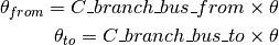
First we compute the arrays of nodal voltage angles for each of the “from” and “to” sides of each branch. This is not a restriction but a simple calculation to aid the next restrictions that apply per branch.

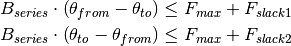
$\theta_{from} = C\_branch\_bus\_{from} \times \theta \theta_{to} = C\_branch\_bus\_{to} \times \theta$

Now, these are restrictions that define that the “from->to” and the “to->from” flows must respect the branch rating.

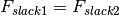
$B_{series} \cdot \left( \theta_{from} - \theta_{to} \right) \leq F_{max} + F_{slack1} B_{series} \cdot \left( \theta_{to} - \theta_{from} \right) \leq F_{max} + F_{slack2}$

Another restriction that we may impose is that the loading slacks must be equal, since they represent the extra line capacity required to transport the power in both senses of the transportation.

$F_{slack1} = F_{slack2}$

Variable	Description	Dimensions	Type	Units
$B_{series}$	Vector of series susceptances of the branches. Can be computed as $Im\left(\frac{1}{r + j \cdot x}\right)$	m	Float	p.u.
$C\_branch\_bus_{from}$	Branch-Bus connectivity matrix at the “from” end of the branches.	m, n	int	1/0
$C\_branch\_bus_{to}$	Branch-Bus connectivity matrix at the “to” end of the branches.	m, n	int	1/0
$\theta_{from}$	Matrix of bus voltage angles at the “from” end of the branches per bus and time step.	m, nt	LP	radians.
$\theta_{to}$	Matrix of bus voltage angles at the “to” end of the branches per bus and time step.	m, nt	LP	radians.
$\theta$	Matrix of bus voltage angles per bus and time step.	n, nt	LP	radians.
$F_{max}$	Matrix of branch ratings per branch and time step.	m, nt	Float	p.u.
$F_{slack1}$	Matrix of branch rating slacks in the from->to sense per branch and time step.	m, nt	LP	p.u.
$F_{slack2}$	Matrix of branch rating slacks in the to->from sense per branch and time step.	m, nt	LP	p.u.

Battery discharge restrictions¶

The first value of the batteries’ energy is the initial state of charge ( $SoC_0$ ) times the battery capacity.

$E_0 = SoC_0 \cdot Capacity$

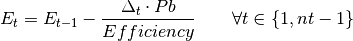
The capacity in the subsequent time steps is the previous capacity minus the power dispatched. Note that the convention is that the positive power is discharged by the battery and the negative power values represent the power charged by the battery.

$E_t = E_{t-1} - \frac{\Delta_t \cdot Pb}{Efficiency} \quad \quad \forall t \in \{ 1, nt-1 \}$

The batteries’ energy has to be kept within the batteries’ operative ranges.

$SoC_{min} \cdot Capacity \leq E_t \leq SoC_{max} \cdot Capacity \quad \forall t \in \{ 0, nt-1 \}$

Variable	Description	Dimensions	Type	Units
$E$	Matrix of energy stored in the batteries.	nb, nt	LP	p.u.
$SoC_0$	Vector of initial states of charge.	nb	Float	p.u.
$SoC_{max}$	Vector of maximum states of charge.	nb	Float	p.u.
$SoC_{min}$	Vector of minimum states of charge.	nb	Float	p.u.
$Capacity$	Vector of battery capacities.	nb	Float	h $\left(\frac{MWh}{MW \quad base} \right)$
$\Delta_t$	Time increment in the interval [t-1, t].	1	Float
$Pb$	Vector of battery power injections.	nb	LP	p.u.
$Efficiency$	Vector of Battery efficiency for charge and discharge.	nb	Float	p.u.

[1]	Rossoni, P. / Moreti da Rosa, W. / Antonio Belati, E., Linearized AC Load Flow Applied to Analysis in Electric Power Systems, IEEE Latin America Transactions, 14, 9; 4048-4053, 2016