Newton-Raphson
All the explanations on this section are implemented here.
Canonical Newton-Raphson
The Newton-Raphson method is the standard power flow method tough at schools. GridCal implements slight but important modifications of this method that turns it into a more robust, industry-standard algorithm. The Newton-Raphson method is the first order Taylor approximation of the power flow equation.
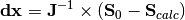
The expression to update the voltage solution in the Newton-Raphson algorithm is the following:

Where:
 : Voltage vector at the iteration t (current voltage).
 : Voltage vector at the iteration t+1 (new voltage).
 : Jacobian matrix.
 : Specified power vector.
 : Calculated power vector using .
In matrix form we get:
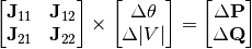
Jacobian in power equations
The Jacobian matrix is the derivative of the power flow equation for a given voltage set of values.
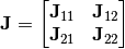
Where:
![J11 = Re\left(\frac{\partial \textbf{S}}{\partial \theta}[pvpq, pvpq]\right)](../../_images/math/71cded0be23ddd29d335c6454c130b359e0080ef.png)
![J12 = Re\left(\frac{\partial \textbf{S}}{\partial |V|}[pvpq, pq]\right)](../../_images/math/ce92e3156ac851d1d4287d32b8eb2ec720389d65.png)
![J21 = Im\left(\frac{\partial \textbf{S}}{\partial \theta}[pq, pvpq]\right)](../../_images/math/85e859d49a236faf8f3d7ed0a417a9c9c9bdf6f0.png)
![J22 = Im\left(\frac{\partial \textbf{S}}{\partial |V|}[pq pq]\right)](../../_images/math/4283fd28a8486dedb125622cb9addf813b2248d5.png)
Where:

Here we introduced two complex-valued derivatives:


Where:
 : Diagonal matrix formed by a voltage solution.
 : Diagonal matrix formed by a voltage solution, where every voltage is divided by its module.
 : Diagonal matrix formed by the current injections.
 : And of course, this is the circuit full admittance matrix.
This Jacobian form can be used for other methods.
Newton-Raphson-Iwamoto
In 1982 S. Iwamoto and Y. Tamura present a method [1] where the Jacobian matrix J is only computed at the beginning, and the iteration control parameter µ is computed on every iteration. In GridCal, J and µ are computed on every iteration getting a more robust method on the expense of a greater computational effort.
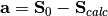
The Iwamoto and Tamura’s modification to the Newton-Raphson algorithm consist in finding an optimal acceleration parameter µ that determines the length of the iteration step such that, the very iteration step does not affect negatively the solution process, which is one of the main drawbacks of the Newton-Raphson method:

Here µ is the Iwamoto optimal step size parameter. To compute the parameter µ we must do the following:
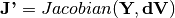
The matrix  is the Jacobian matrix computed using
the voltage derivative numerically computed as the voltage increment
is the Jacobian matrix computed using
the voltage derivative numerically computed as the voltage increment
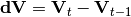 (voltage difference between the
current and the previous iteration).
(voltage difference between the
current and the previous iteration).

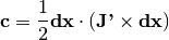

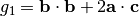


There will be three solutions to the polynomial  . Only the last solution
will be real, and therefore it is the only valid value for
. Only the last solution
will be real, and therefore it is the only valid value for  . The polynomial
can be solved numerically using 1 as the seed.
. The polynomial
can be solved numerically using 1 as the seed.
| [1] | Iwamoto, S., and Y. Tamura. “A load flow calculation method for ill-conditioned power systems.”IEEE transactions on power apparatus and systems 4 (1981): 1736-1743. |
Newton-Raphson Line Search
The method consists in adding a heuristic piece to the Newton-Raphson routine. This heuristic rule is to set µ=1, and decrease it is the computed error as a result of the voltage update is higher than before. The logic here is to decrease the step length because the update might have gone too far away. The proposed rule is to divide µ by 4 every time the error increases. There are more sophisticated ways to achieve this, but this rule proves to be useful.
The algorithm is then:
Start.
Compute the power mismatch vector
using the initial voltage solution
.
Compute the error. Equation ref{eq:nr_error}.
While
or
:
Compute the Jacobian
Solve the linear system.
Set
.
Assign
to
Compute the power mismatch vector
Compute the error.
If the
from the previous iteration:
g1. Decrease
g2. Assign
g3. Compute the power mismatch vector
g4. Compute the error.
End.


The Newton-Raphson method tends to diverge if the grid is not
perfectly balanced in loading and well conditioned (i.e.: the impedances are not wildly
different in per unit and X>R). The control parameter  turns the
Newton-Raphson method into a more controlled method that converges
in most situations.
turns the
Newton-Raphson method into a more controlled method that converges
in most situations.
Newton-Raphson in Current Equations
Newton-Raphson in current equations is similar to the regular Newton-Raphson algorithm presented before, but the mismatch is computed with the current instead of power.
The Jacobian is then:
![J=
\left[
\begin{array}{cc}
Re\left\{\left[\frac{\partial I}{\partial \theta}\right]\right\}_{(pqpv, pqpv)} &
Re\left\{\left[\frac{\partial I}{\partial Vm}\right]\right\}_{(pqpv, pq)} \\
Im\left\{\left[\frac{\partial I}{\partial \theta}\right]\right\}_{(pq, pqpv)} &
Im\left\{\left[\frac{\partial I}{\partial Vm}\right]\right\}_{(pq,pq)}
\end{array}
\right]](../../_images/math/d561f8db1cbcd61577d7e8dec79873eb63c3ffd6.png)
Where:
![\left[\frac{\partial I}{\partial Vm}\right] = [Y] \times [E_{diag}]](../../_images/math/940ee2d9a04de6400f004e6a8b3a5f7e42b49857.png)
![\left[\frac{\partial I}{\partial \theta}\right] = 1j \cdot [Y] \times [V_{diag}]](../../_images/math/ec4479a2b9ddd5ff9ae42b33c1c72666ac8f9cbe.png)
The mismatch is computed as increments of current:
![F = \left[
\begin{array}{c}
Re\{\Delta I\} \\
Im\{\Delta I\}
\end{array}
\right]](../../_images/math/b273904cbb4a463281cbf1dabf125a671c8d7cad.png)
Where:
![[\Delta I] = \left( \frac{S_{specified}}{V} \right)^* - ([Y] \times [V] - [I^{specified}])](../../_images/math/8f707bc4dc39a448fcd7a34efa3218ebef7812e0.png)
The steps of the algorithm are equal to the the algorithm presented in Newton-Raphson.